Tutorial: data analysis
In this tutorial, we are going to create a pipeline for processing data stored in an Experiment.
The tutorial project
In this tutorial we use the same dataset as in the first tutorial (see Tutorial: data management). We then suppose that we already have a created experiment with the imported and annotated data.
In the following of this tutorial, we are going to process the data in 3 steps.
Image deconvolution on each image to ease the spot segmentation
Auto thresholding and particle analysis on the deblurred and denoised images
Statistical testing with the Wilcoxon test to conclude if the two populations have significantly different number of spots
The 3 proposed steps are just one possible way to analyse the data. The purpose here is just to illustrate how to use the BioImageIT app. Many other processing pipeline are possible to analyse this dataset, but it is not the purpose of this tutorial.
First, we open the BioImageIT application:
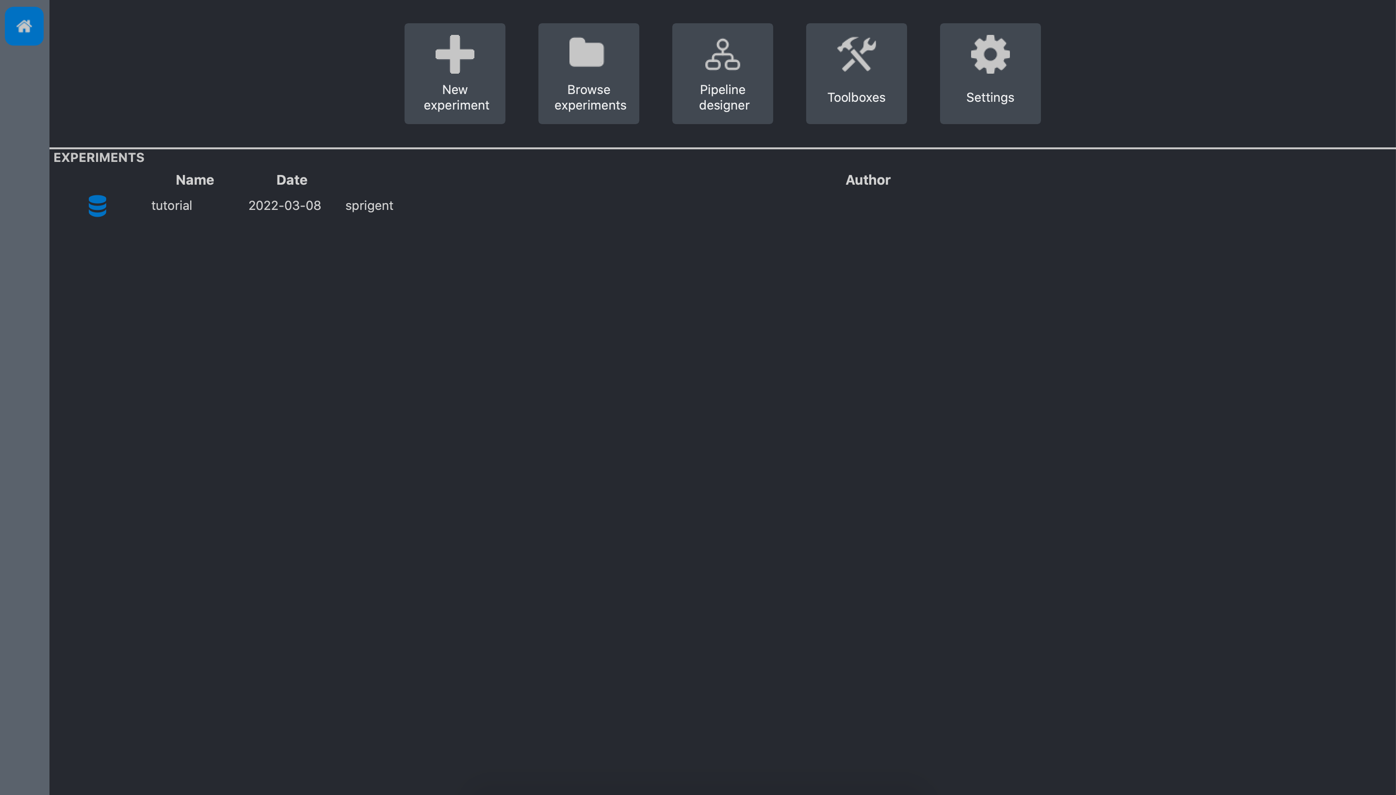
Image deconvolution
To ease the spot segmentation, we chose to preprocess the data with a deconvolution algorithm. The selected algorithm is the Spitfire2D. It is a c++ implementation of a sparse variation deconvolution method.
Click on the Toolboxes button main application top bar:
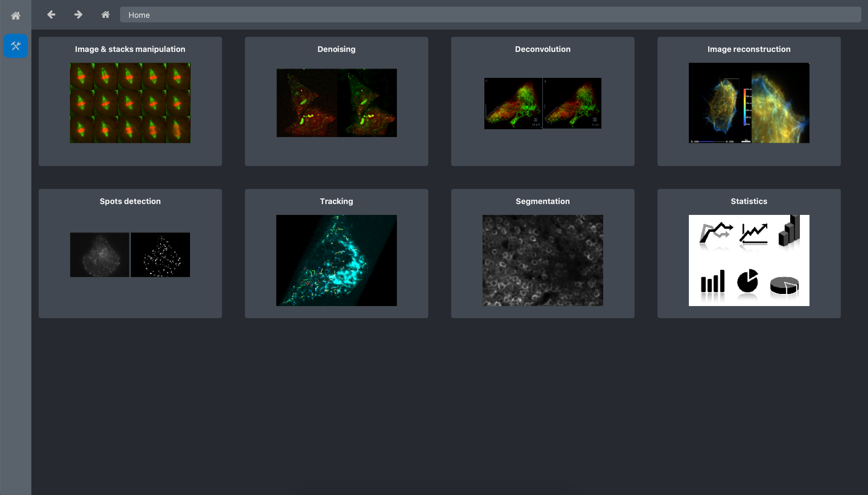
Then click on the Deconvolution toolbox:
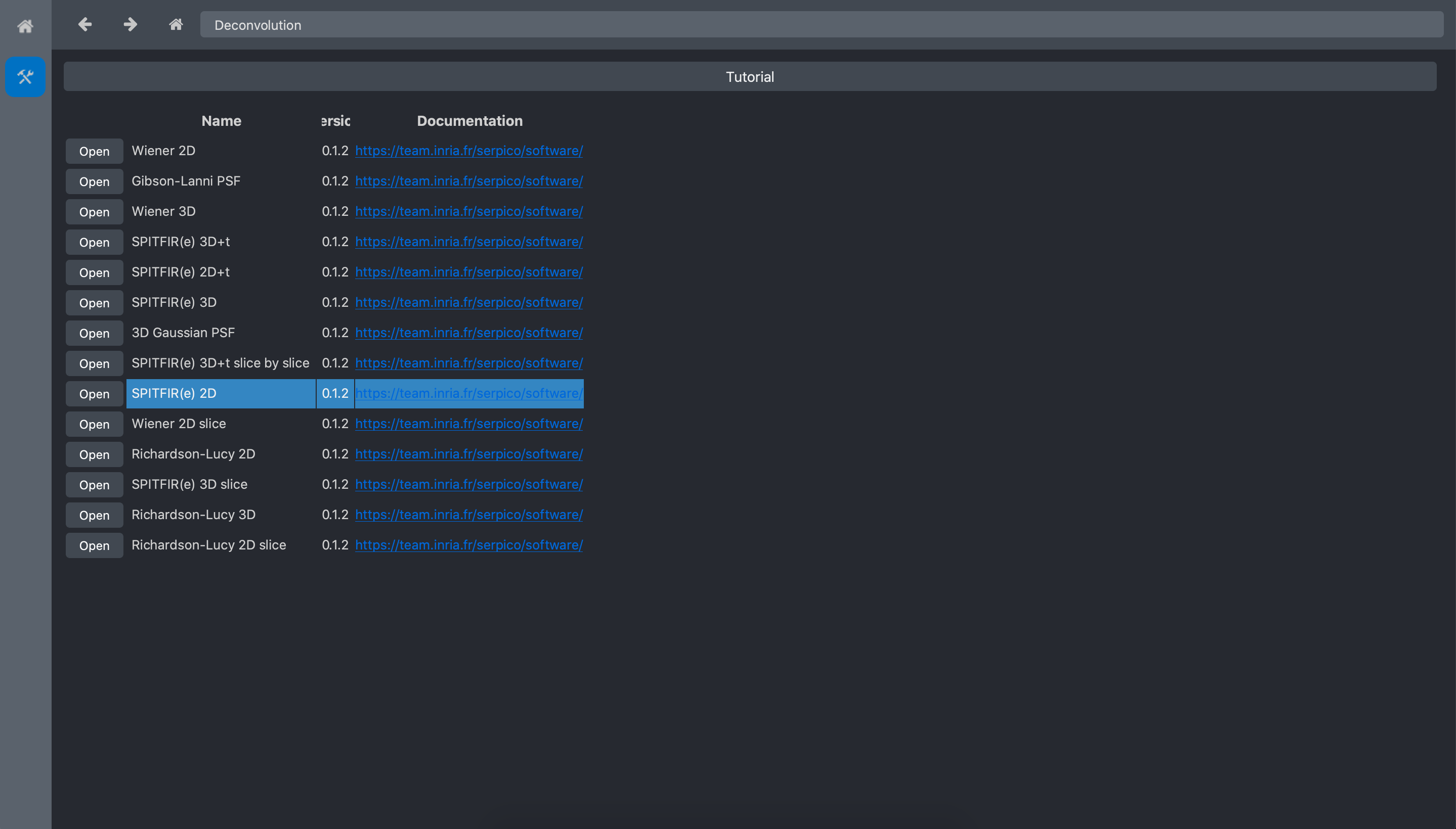
And click on the Spitfire 2D tool open button:
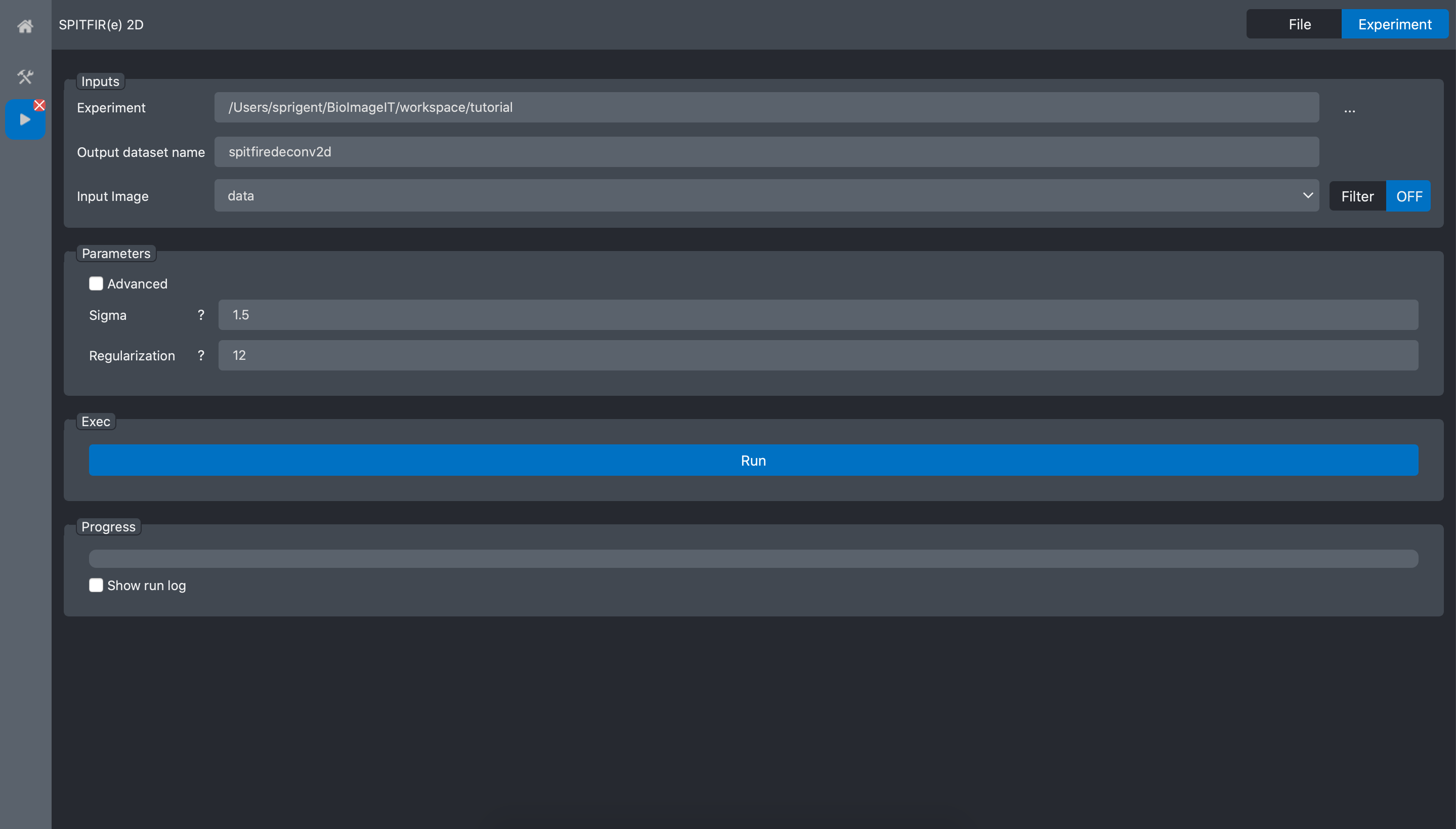
We can now run the tool on the tutorial Experiment. Select the tutorial experiment in the
“Experiment” field. When the experiment is recognised, the field Input image is automatically
filed with the data dataset which is the only dataset we have in our experiment.
Then we need to setup the deconvolution parameters. This task can be done by trial and error. In this example we previously selected the best parameters as:
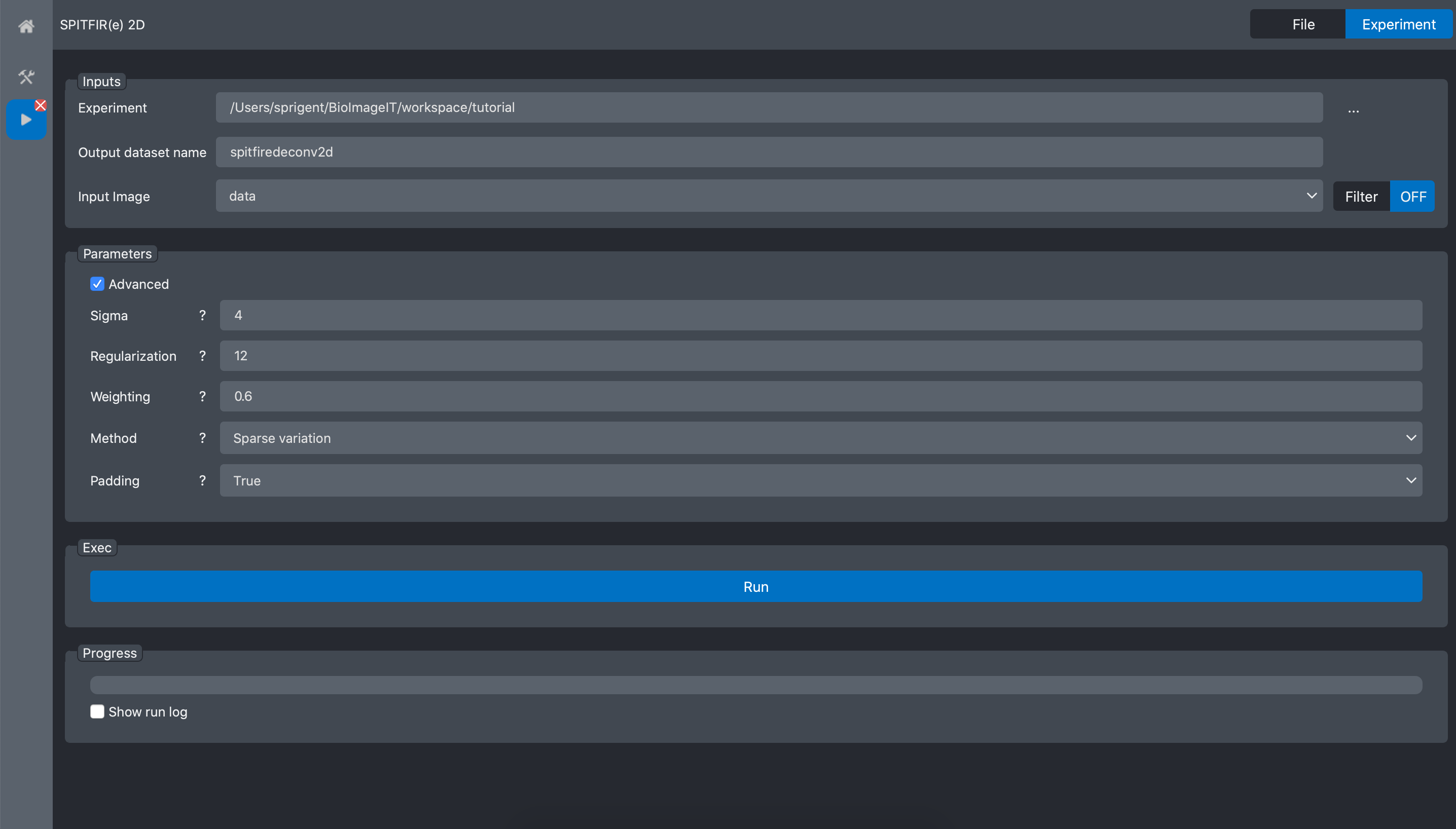
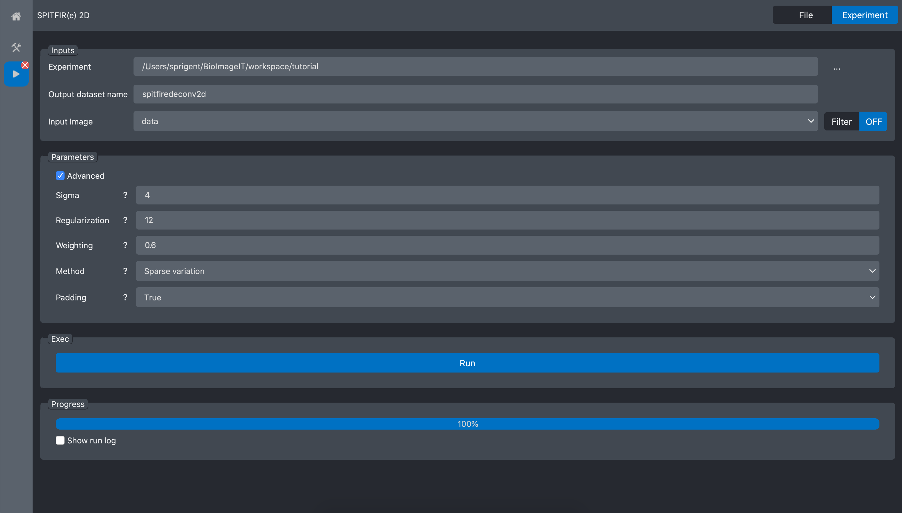
Press Run and wait the process to finish:
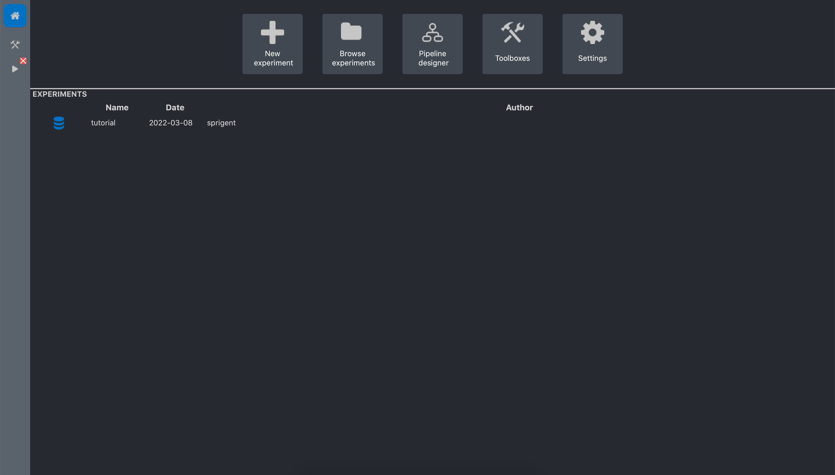
We can now open the experiment from the home page:
And select the spitfiredeconv2d dataset
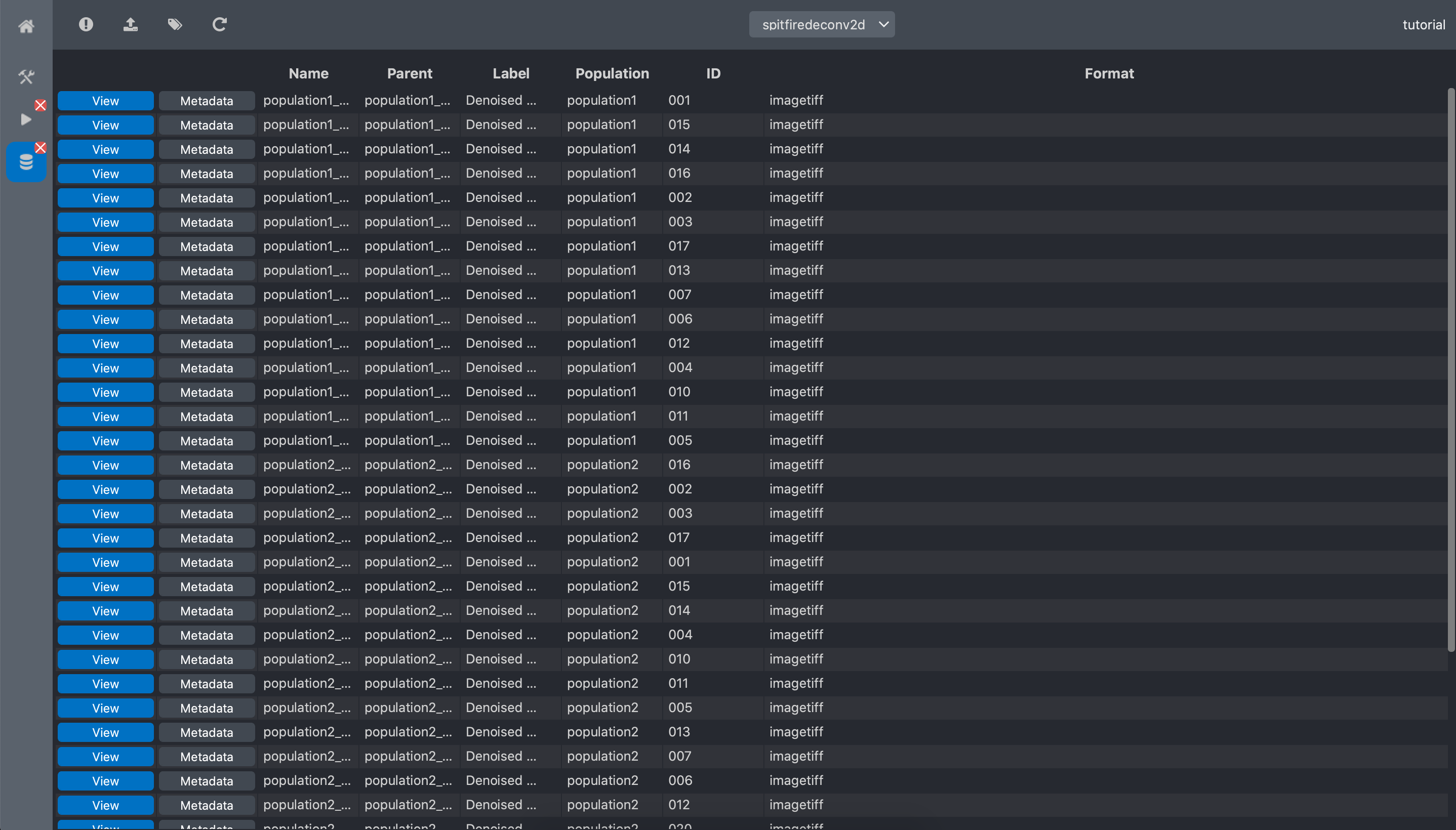
We can visualize the obtained result by clicking the View button of an image:
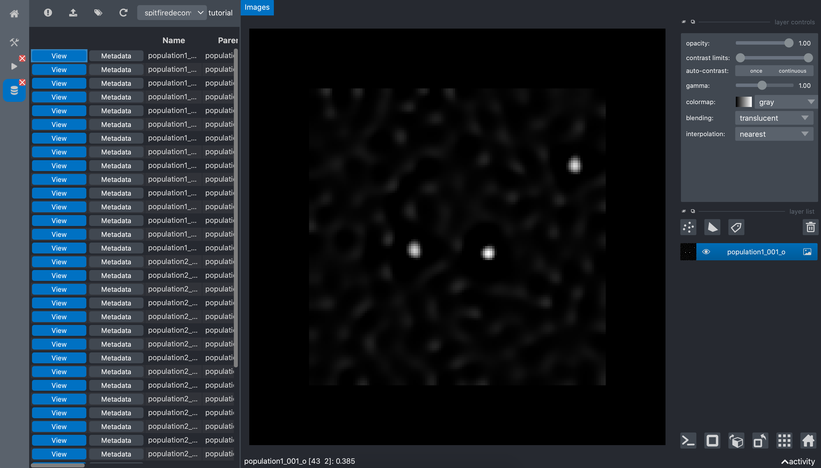
we can see that the sports are now easy to distinguish from the background. The metadata button of each image show the metadata of the image and the details of it origin (raw data annotations and run information).
Spot detection
After deconvolution, the spots are easy to detect on the images. We can simply threshold the image and count the number of independent component in the binary map. BioImageIT wrap a Fiji macro that runs an auto-threshold and the analyse particles tool. This is exactly what we need here.
Open the Toolboxes:
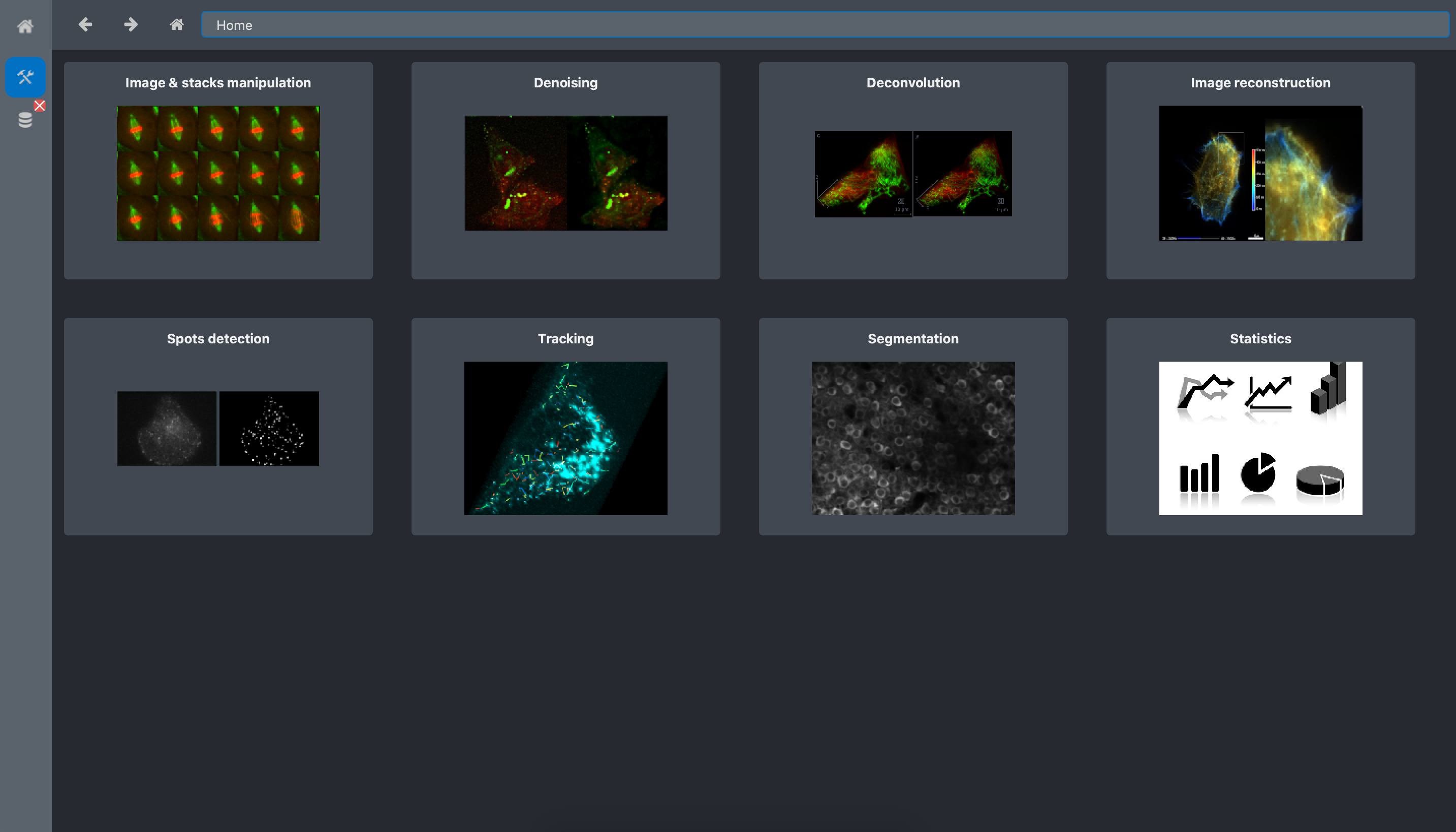
Click on the Spots detection toolbox.
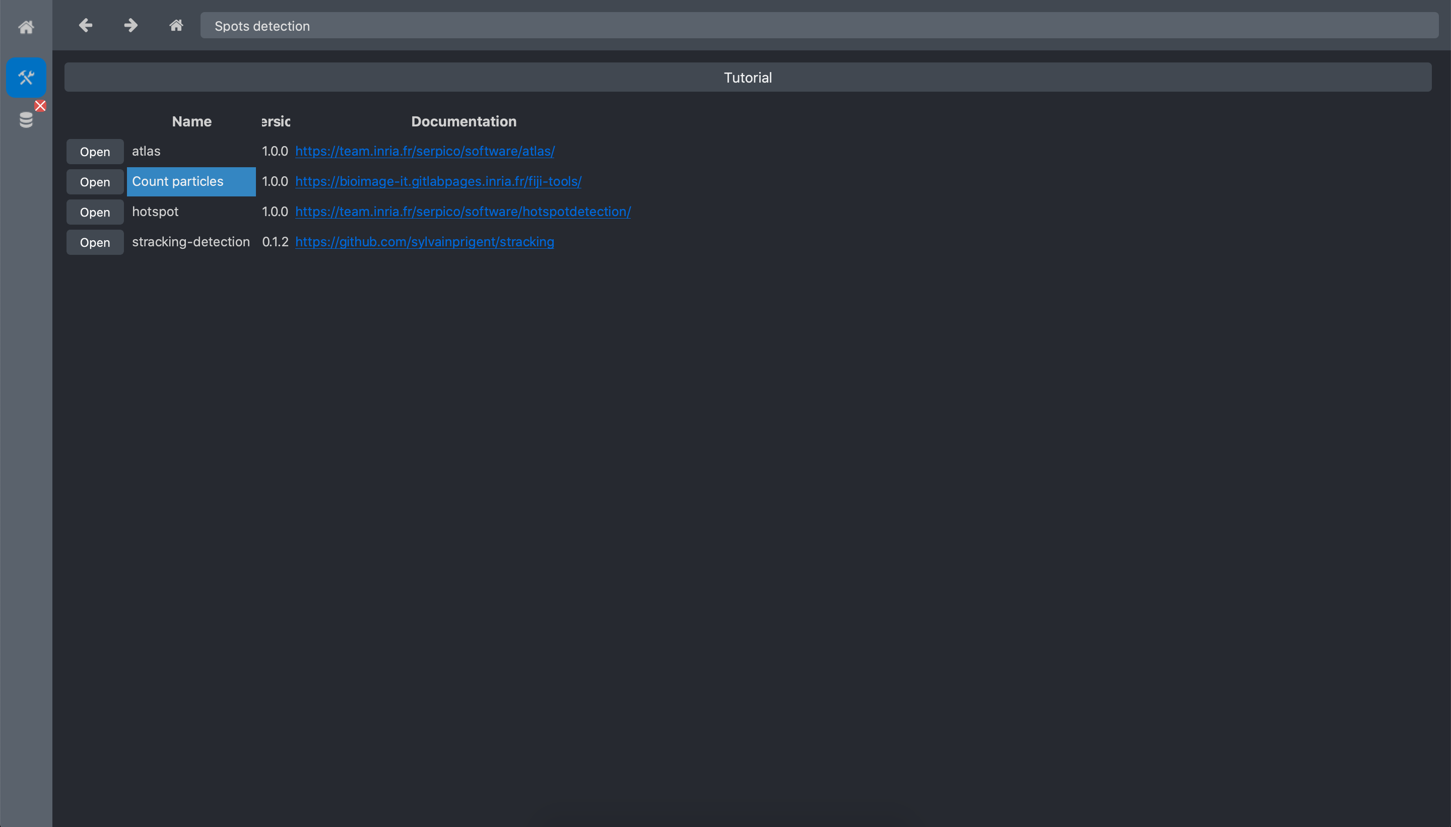
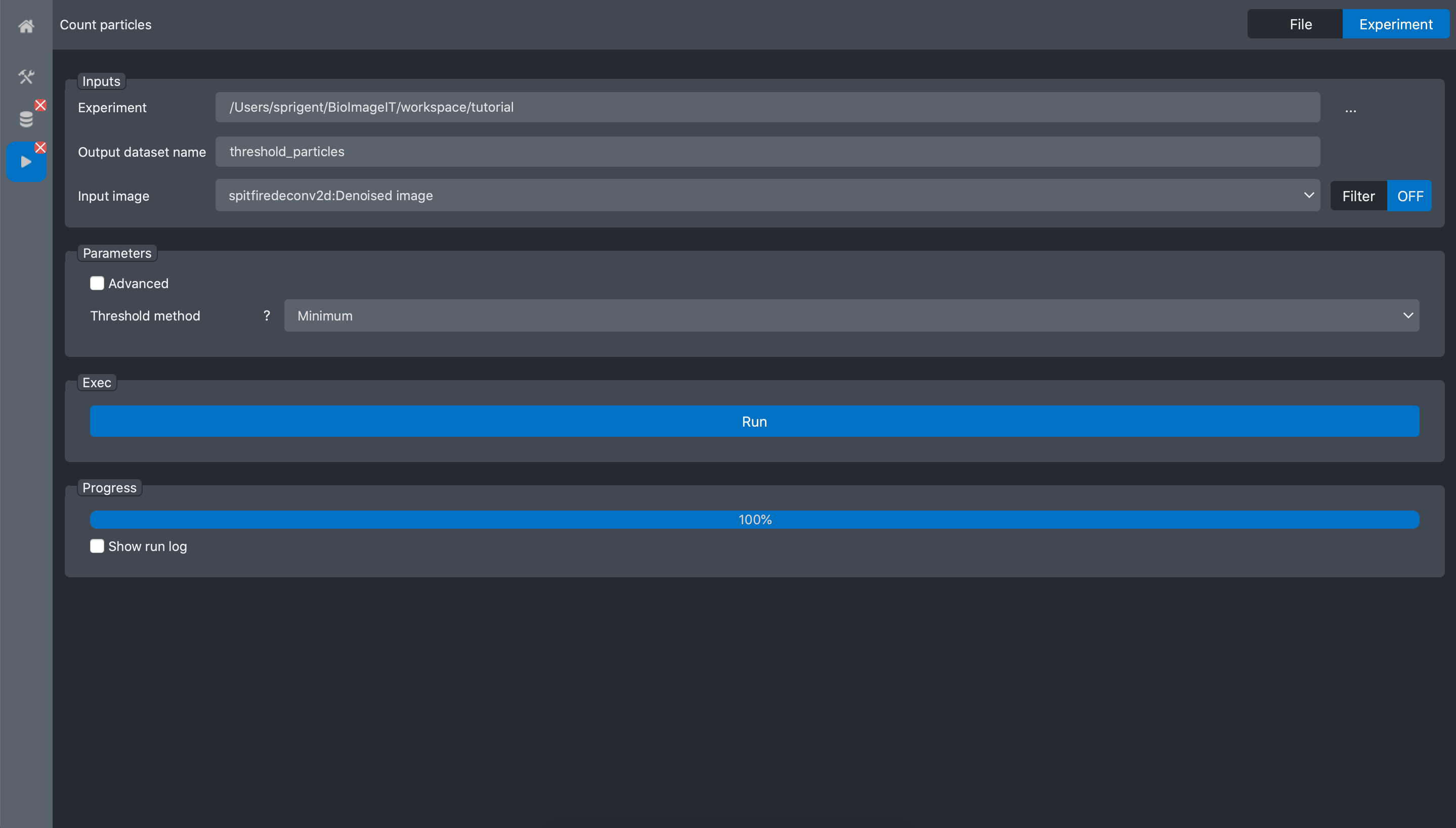
Open the Count particles tool:
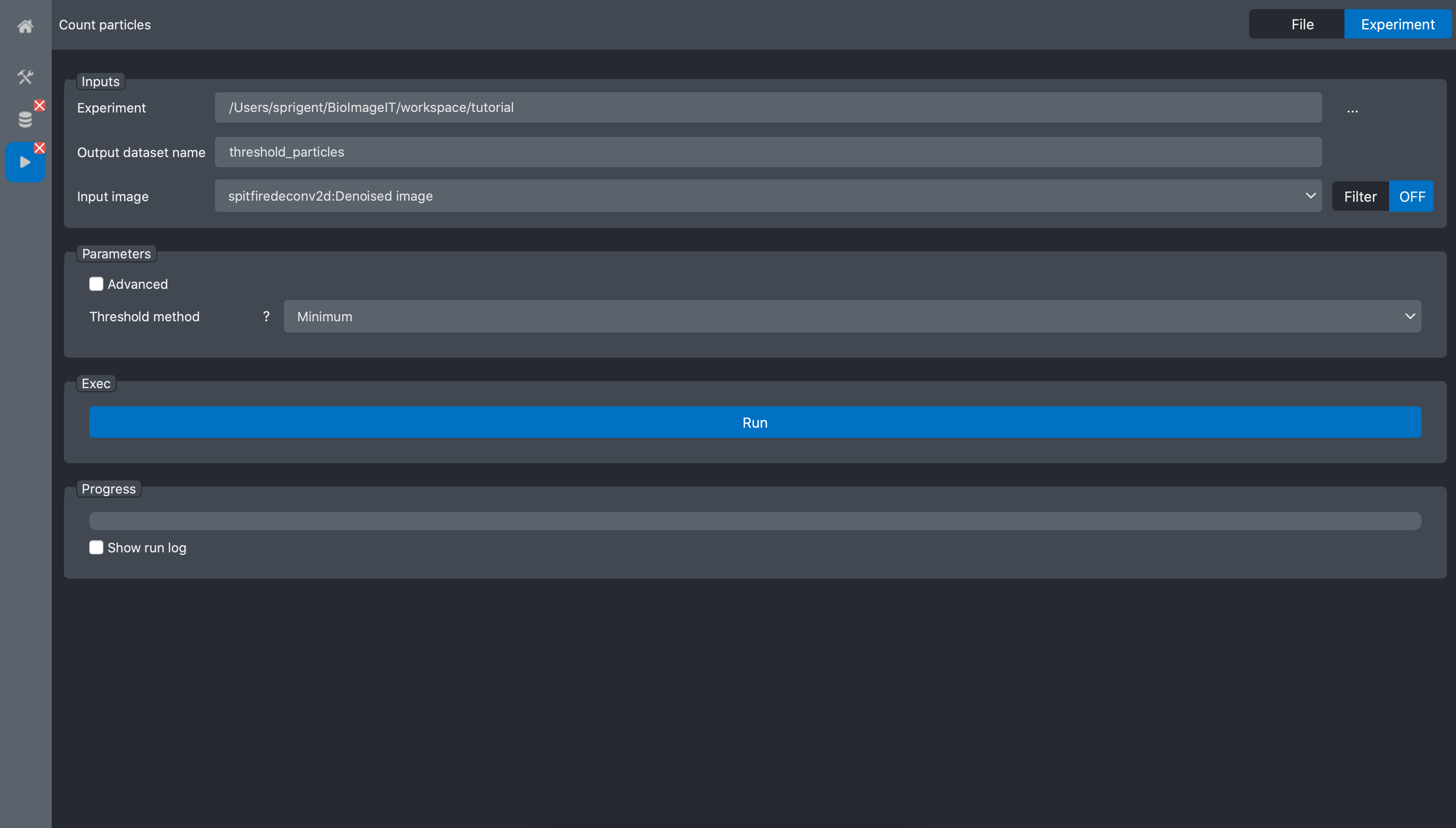
In the experiment field, select the tutorial experiment, and for the input image field
select the deconvolution image from the previous process: spitfiredeconv2d:Denoised image
Press Run and wait for the process to finish:
We can now go back to the experiment editor tab, and press the refresh button for the new dataset
threshold particles to appear.
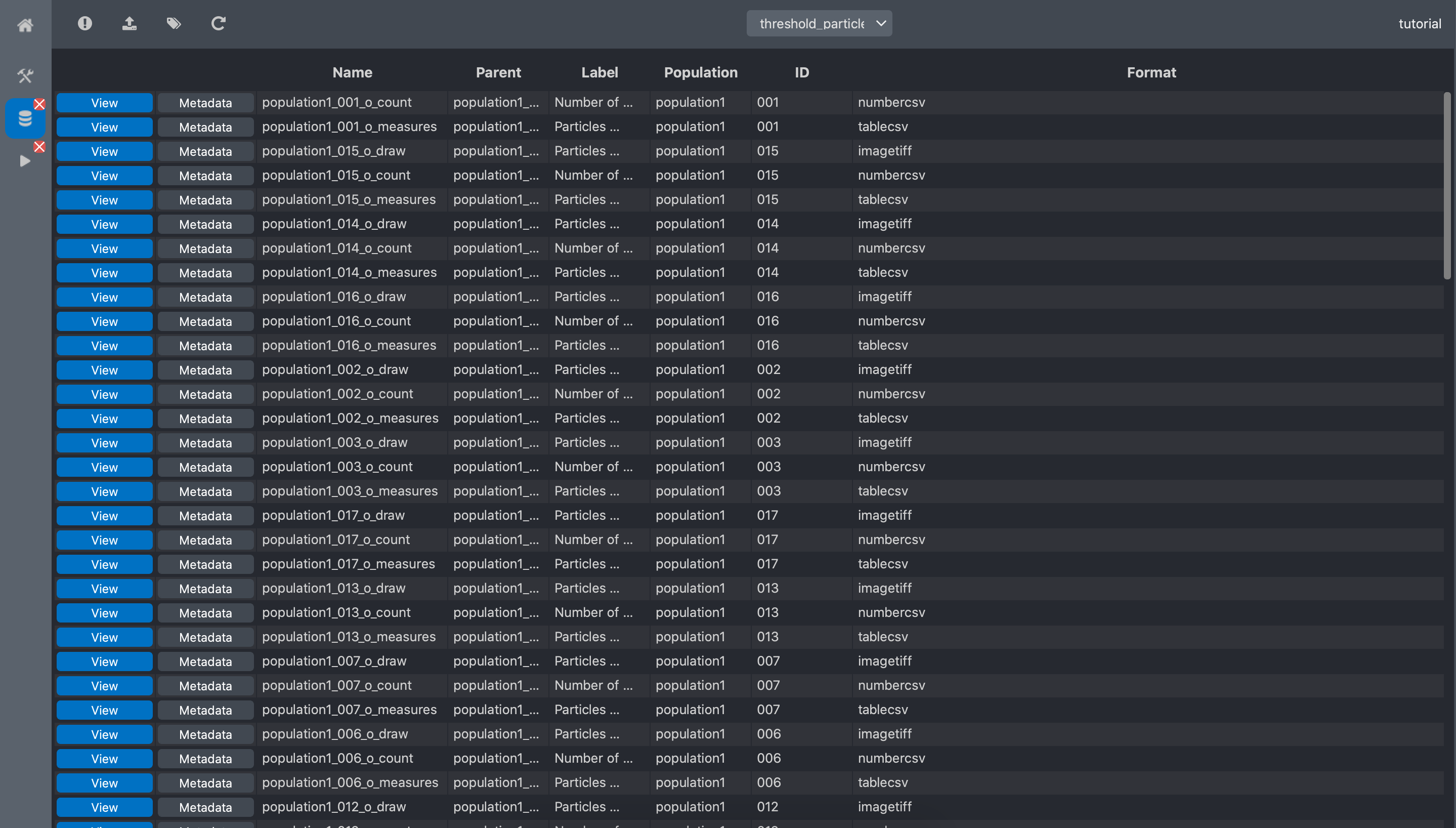
We can see that we have 3 new data per image: count, measure, draw. count is the
number of spot in the image. It is the output of interest for our problem. measure is a table
with properties of the spots and draw is a representation of the spot localisation.
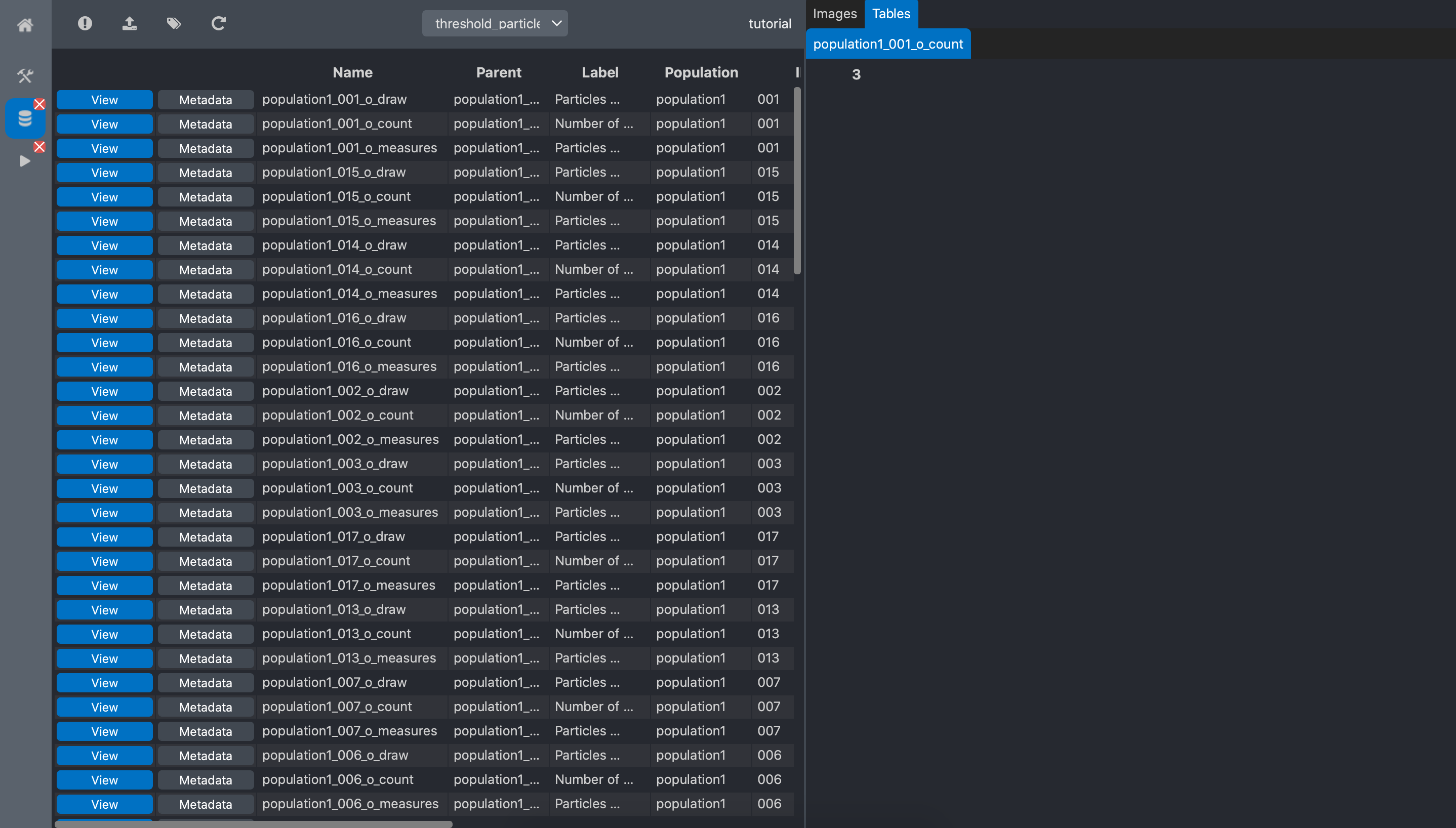
If we click on the view button of the count data, the viewer shows the number of spot for
this image:
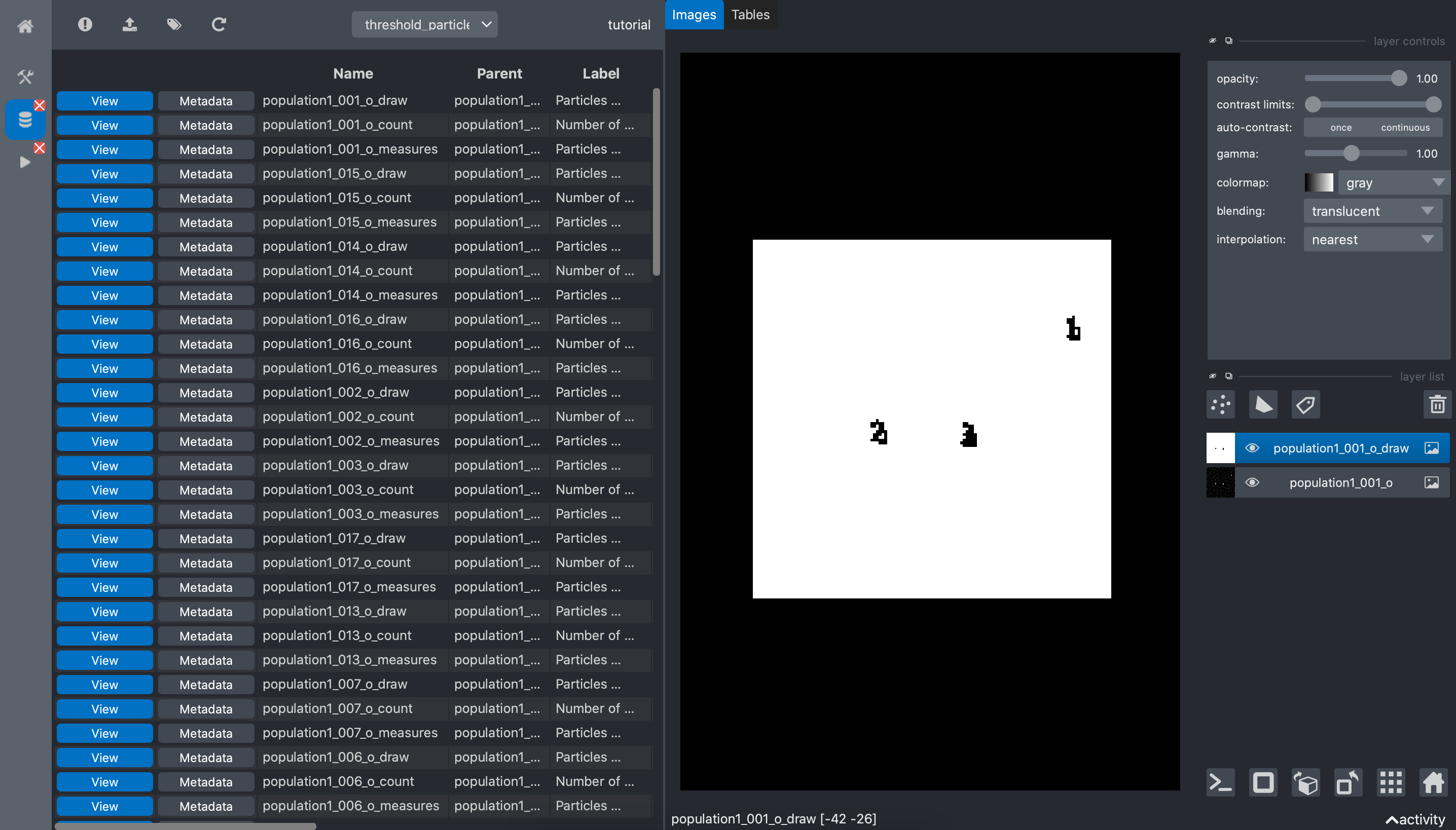
And clicking on the view button of the count data shows the localization of the detected
spots:
Statistical testing
In the previous processing step, we extracted the number of spots for each image. This number is
contained in the count data file for each image. In this step we are going to run a statistical
testing on these number in order to measure if the Population1 and Population2 data have
significant different numbers of spots.
To illustrate the use of statistical testing with BioImageIT, we chose in this tutorial to run a Wilcoxon rank test. This is not the best test for such statistical analysis, but the purpose of the tutorial is to show how to run tools, and Wilcoxon rank test is a simple easy to use example.
Go back to the toolboxes tab of the BioImageIT app,
and select the statistics toolbox:
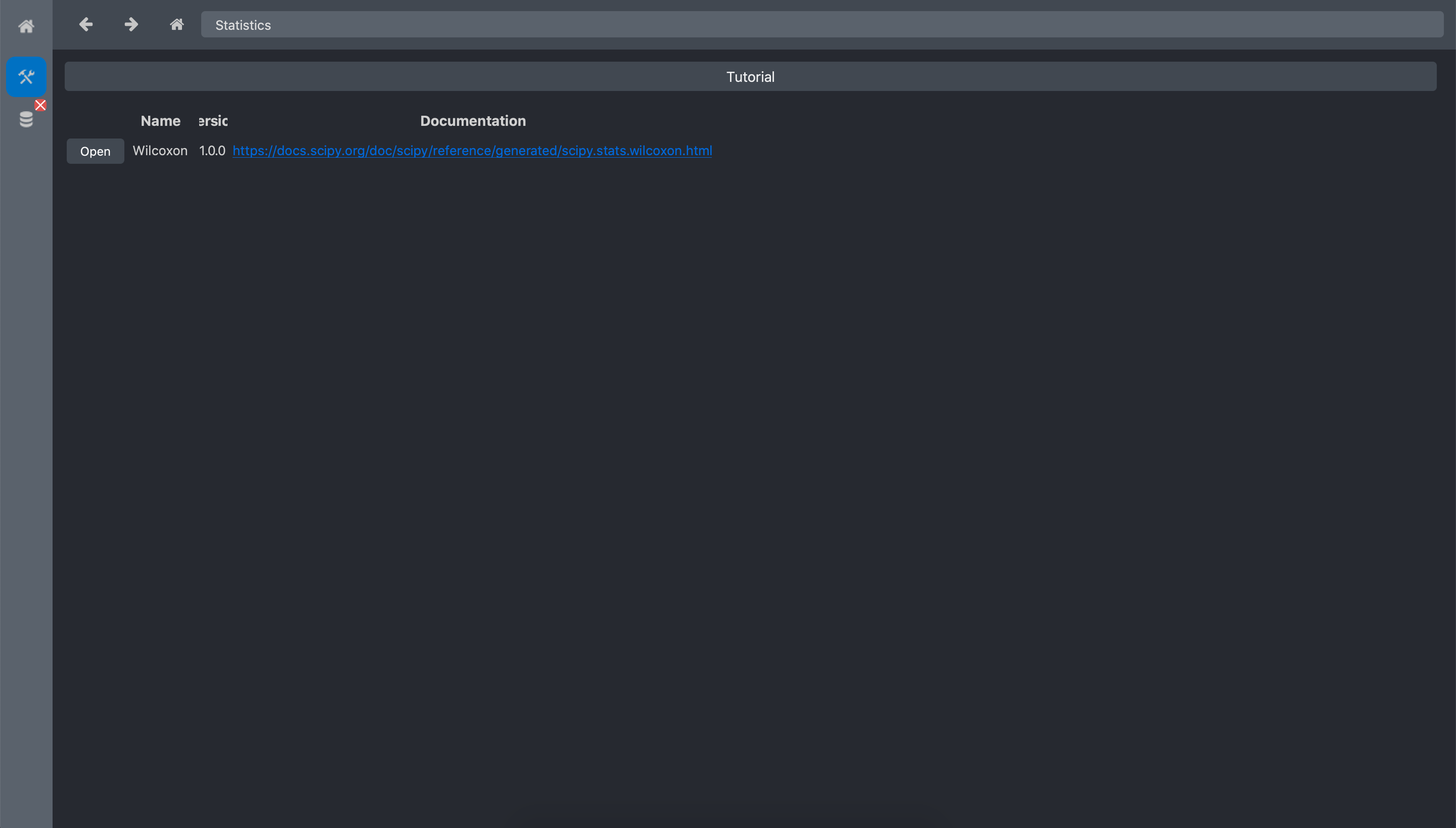
Open the Wilcoxon tool:
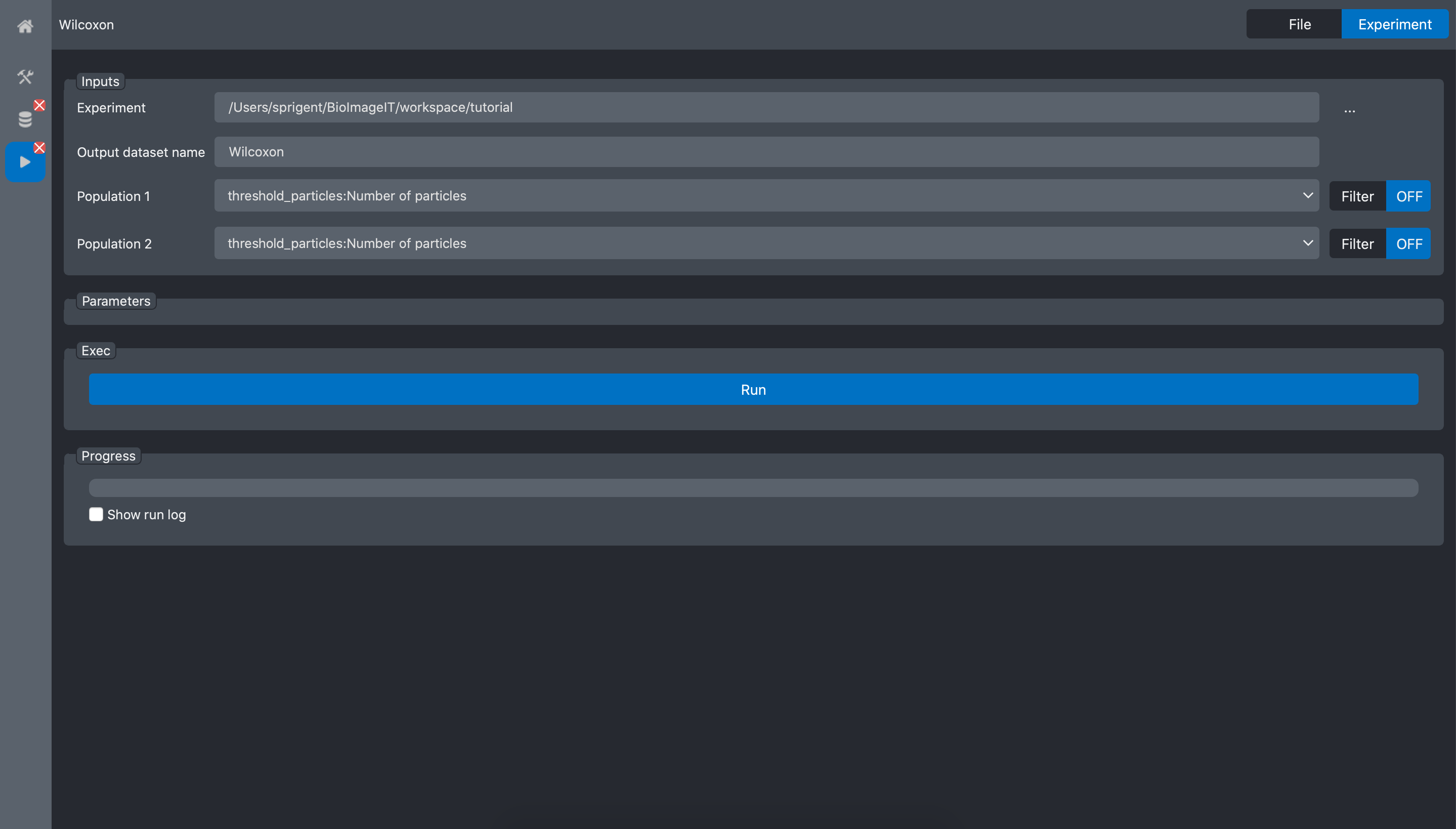
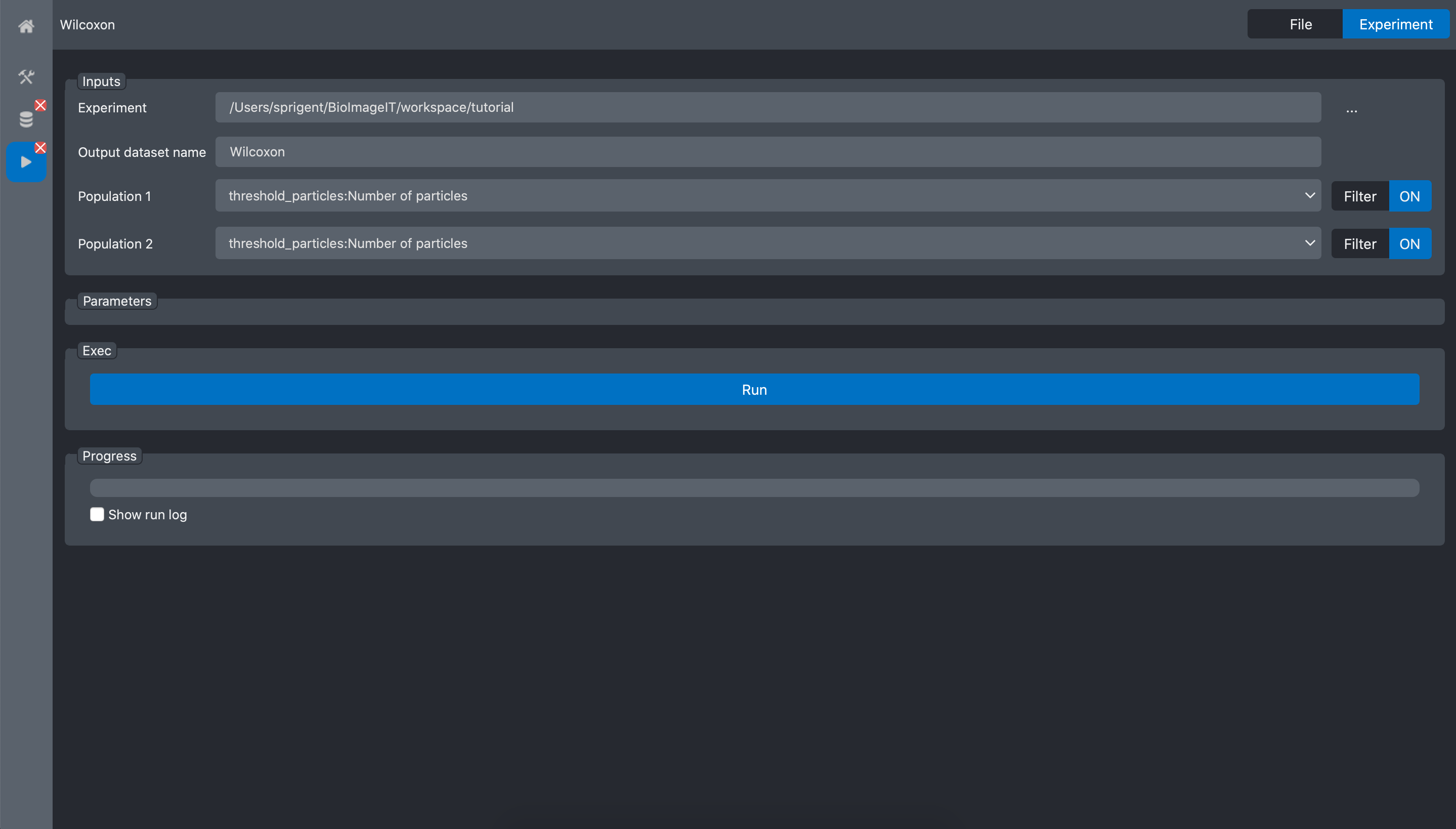
Select the tutorial experiment in the Experiment field.
The Wilcoxon tool have too inputs: Population1 and Population2. These two inputs are in fact arrays of values corresponding to the two populations we want to process. In most of the existing applications, to construct such arrays, we need to write a script that read the values (number of spot) for each image, create the two arrays and run the statistical test.
Because in BioImageIT, we annotated the data, we can simply use Filter to automatically generate the data arrays.
For the Population1 and Population2, select the line threshold_particles:Number Of Particles (see figure above).
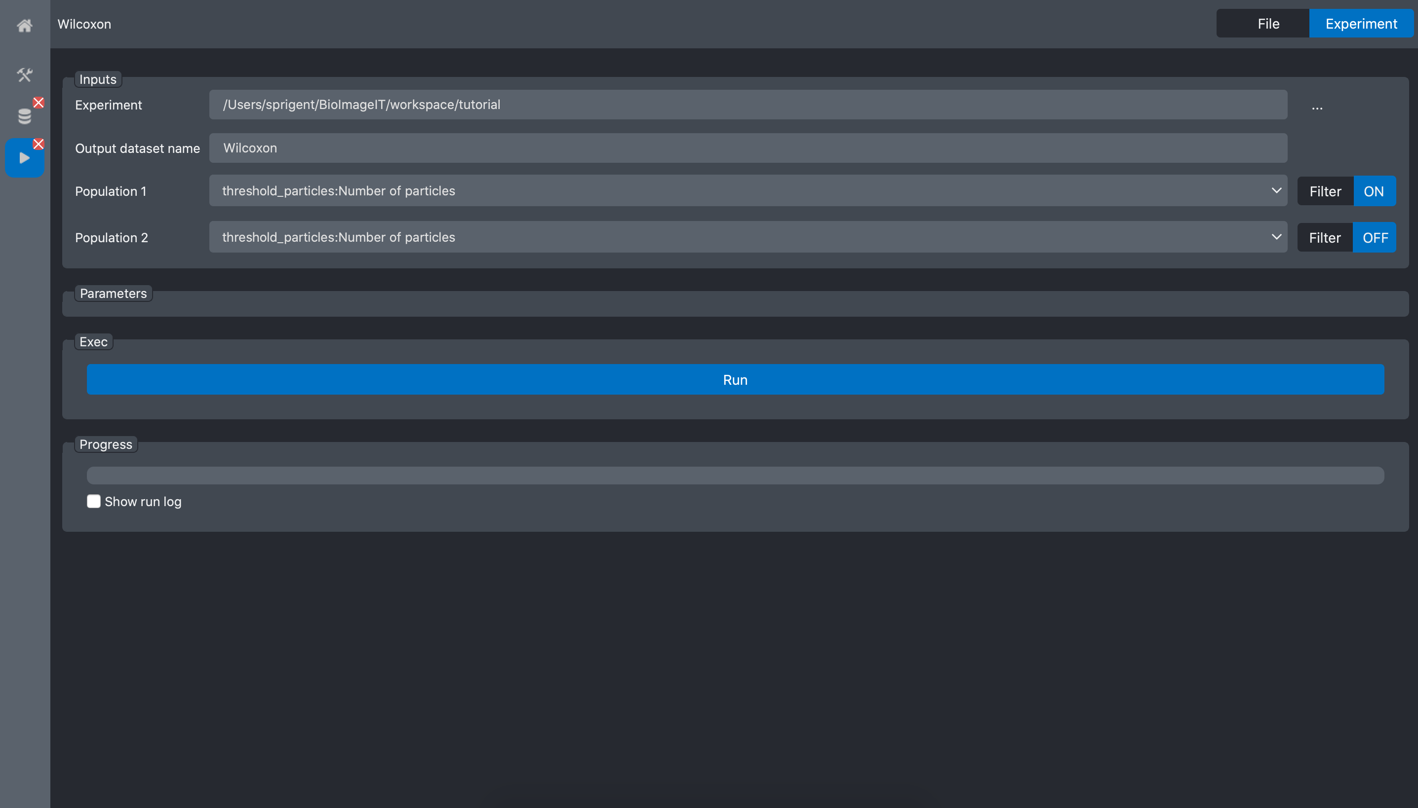
Now, we need to specify that for Population1 we want to select the images with the corresponding key-value pair: Population=population1. Click on the Filter button at the right of the Population1 input. It opens a popup window where you can tune a filter. Here we select the data where the key Population equals “population1”

When we validate, the filters status changes to ON.
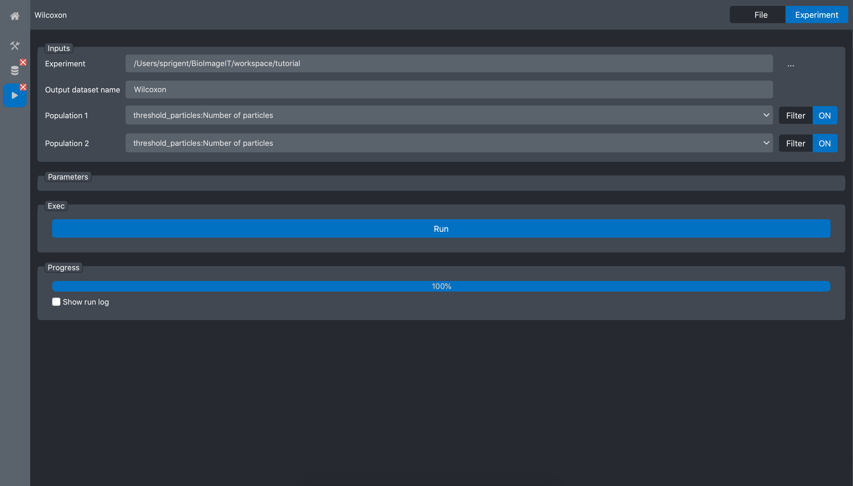
Then, we do the same for the second population:
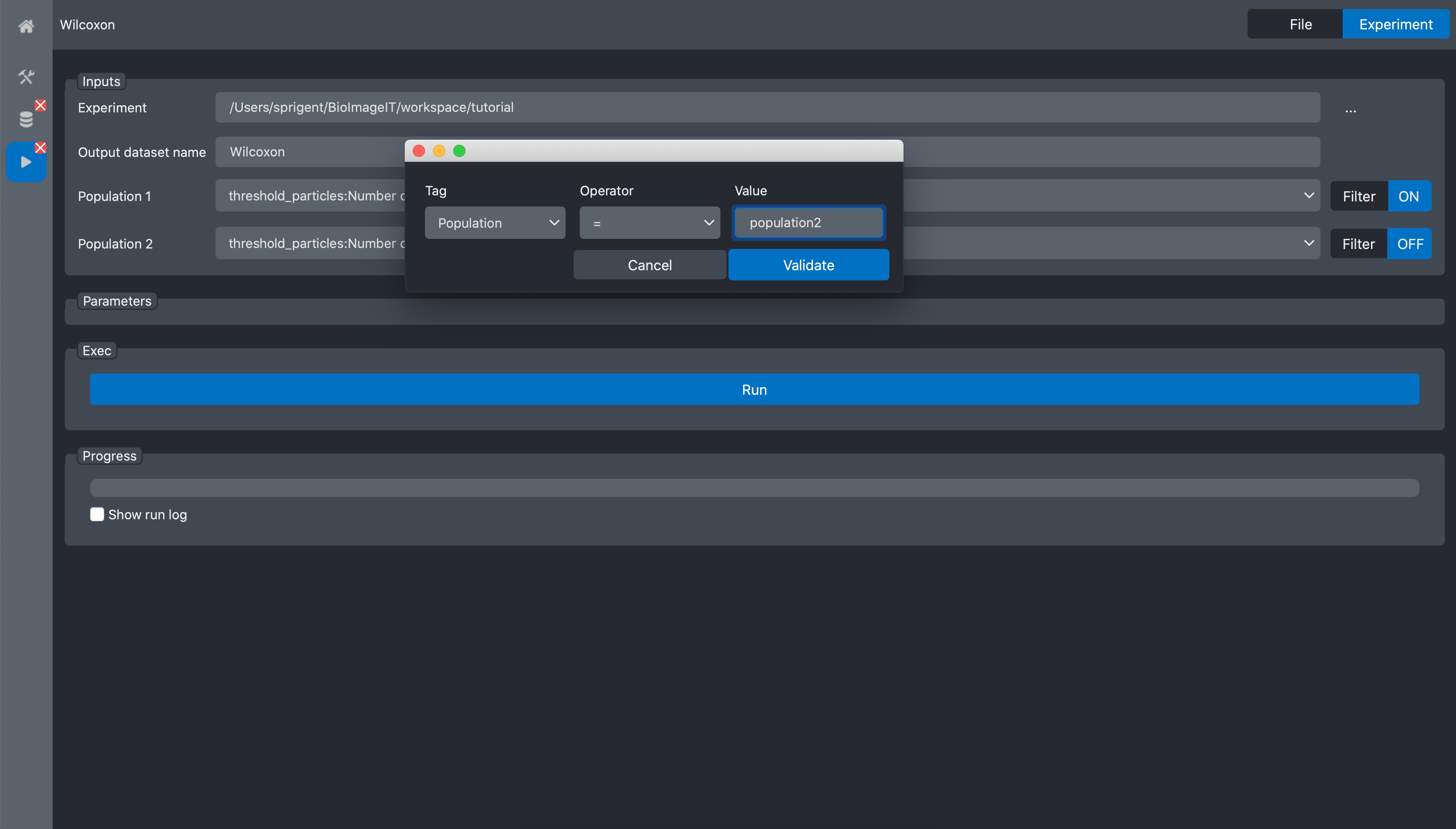
and validate:
Press the Run button:
We can now go to the experiment editor tab, press Refresh on the to toolbar and select the
Wilcoxon dataset:
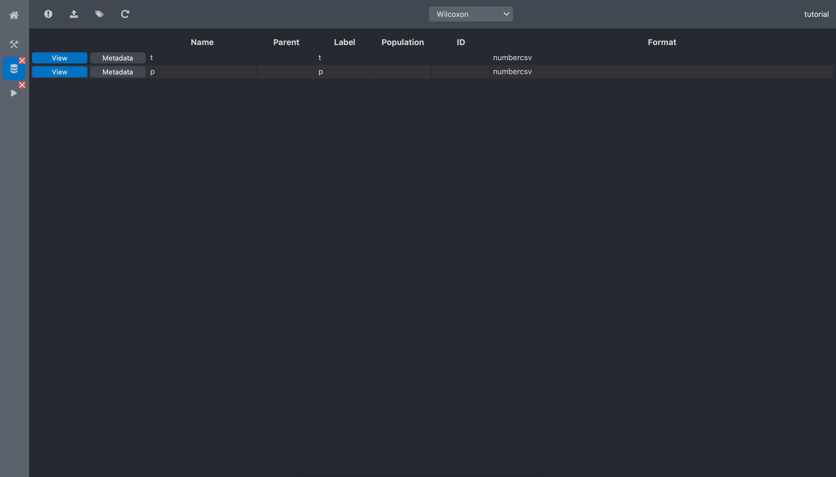
We can now see the Wilcoxon dataset contains 2 data:
t: the Wilcoxon statistic
p: the p-value
Click the view button of the p-value data:
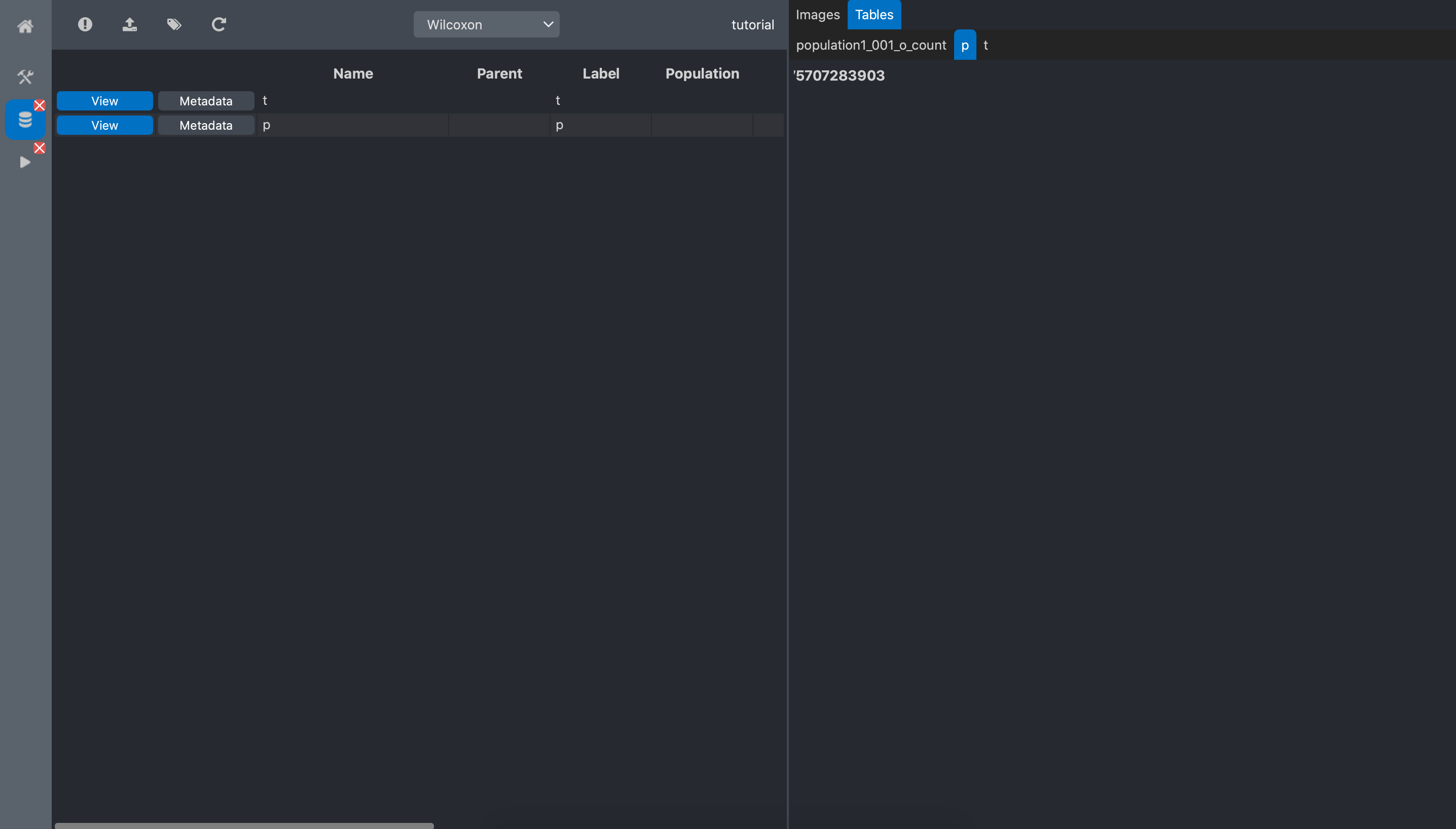
We can read that the p-value equals 0.0075. This means that we can reject the null hypothesis saying that the 2 populations have the same number of spots.
Note
During the step, we mention that BioImageIT created two arrays from the dataset
threshold_particles:Number Of Particles using the Filters that we tuned with the experiment
annotations. In fact, these arrays are stored in the output dataset. Thus, if we open the
directory path/to/tutorial/Wicoxon/ we can find the file x.csv and y.csv that actually
contain these two arrays.
Conclusion
In this tutorial we saw how to use the BioImageIT app, to build step by step an image analysis pipeline without writing a single line of code.
All the data we generated are stored in an Experiment database with automatically generated
metadata. This means that for every data in the Experiment database, we can track it origin and
the parameters of each processing tool used to generate it.